Marching NumPy

The visualisation of numeric data is a key component of computer graphics.
Data is often encountered as numeric values distibuted over a regular space - sometimes volume data are called voxels data. Visualisation of this numeric data is key to the interpretation and/or appreciation of the data. For example:

• medicine: medical imaging such as MRI and CT scanners.
• science: quantum mechanical calculations and data recording.
• cartography: linking data such as height, land usage, etc to map coordinates.
• entertainment: generation of artwork generated terrain and visualsation of metaballs.

An important method for the visualisation of volume data is to calculate an isosurface: a mesh surface that follows as closely as possible where the data crosses a certain level threshold.

This package includes an implementation of the Lorensen Marching Cubes isosurface calculation algorithm using only Python and NumPy methods: MarchingCubesLorensen.marching_cubes_lorensen(). The algorthimn follows these processes:

• Calculate Intersects. For each time that the volume value crosses the level threshold along each axis, interpolate the position of the intersection - this becomes a vertex for the output mesh. Also calculate a unique id for that vertex.
• Assign Types. Consider each corner of the volume unit and whether it is above or below the level threshold. Assign a unique identifier to each unit based upon the outcome of these logical binary tests. For a cube there are 8 vertices that gives 256 possible outcomes [that are related to a set of 15 core geometries by symmetry].
• Look Up Geometry. Use the calculated type to index a precalculated geometry table the defines how the calculated vertices should be joined using triangular geometry.

Example usage:

>>> import numpy
>>> volume = numpy.load("example_data/test_volume.npy")
>>> import MarchingNumPy
>>> vertices,triangles = MarchingNumPy.marching_cubes_lorensen(volume, level=0.05)
>>> vertices.shape
(4138, 3)
>>> triangles.shape
(8244, 3)

The image below - a molecular orbital of caffeine (pink and green wireframe) - was generated in Blender using the output of this function.

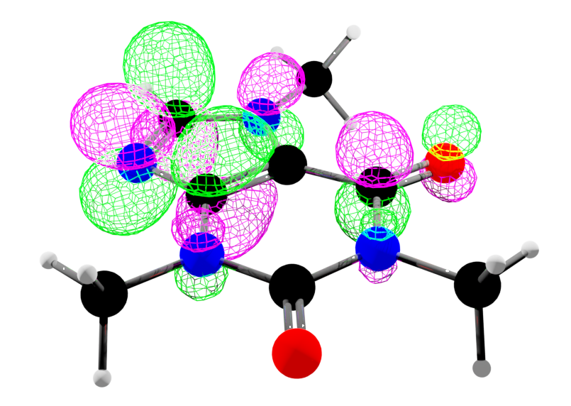
This volume data test_volume.npy is from the Cubefile package.

Hotplates

The MSHPro is low-cost hotplate stirrer.

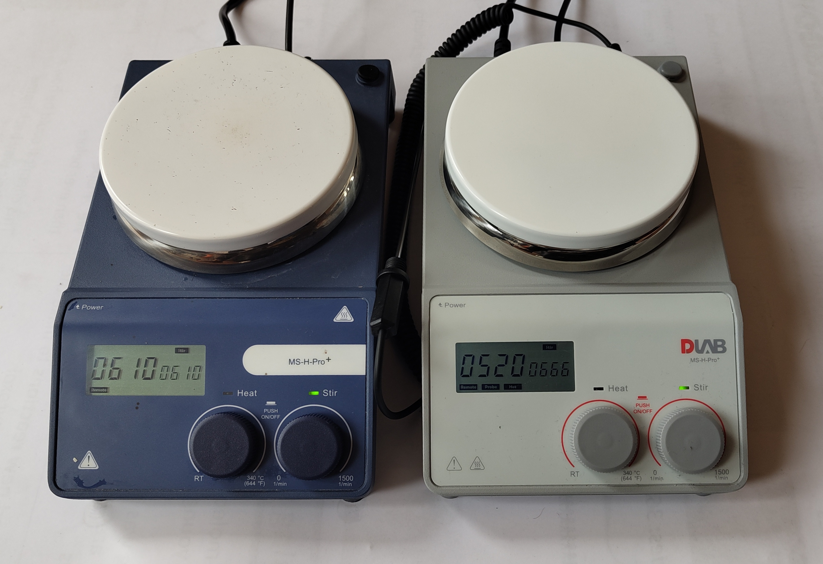
The hotplate has a RS232 9-pin connector on the rear that allows control of its functions. This package is a tool for control of these hotplates via serial interface.

This package is an interface to all commands provided by the Hotplates.MSHPro class.
Commands are avilable to get information and control the hotplate's speed and temperature.
All the formal communication structure is described by the Hotplates.MSHProCommunication module.

Example usage:

>>> import Hotplates
>>> hp = Hotplates.MSHPro(port="/dev/ttyUSB0")
>>> hp.status()
{'success': True, 'stir_set': 'Off', 'stir_actual': 0, 'heat_set': 'Off', 'heat_actual': 17.5, 'stir_on': False, 'heat_on': False, 'heat_limit': 340.0}
>>> hp.stir(400)  # Wait after command for hotplate to reach speed
>>> hp.status()
{'success': True, 'stir_set': 400, 'stir_actual': 399, 'heat_set': 'Off', 'heat_actual': 17.7, 'stir_on': True, 'heat_on': False, 'heat_limit': 340.0}
>>> hp.off()
>>> hp.status()
{'success': True, 'stir_set': 'Off', 'stir_actual': 0, 'heat_set': 'Off', 'heat_actual': 1.1, 'stir_on': False, 'heat_on': False, 'heat_limit': 340.0}

Serial communication is full duplex and this is acheived using Hotplates.SerialThreadedDuplex.Serial, an extension of PySerial's serial.Serial.

Cubefile

.cube files are generated from quantum mechanical chemistry calculations. They contain data about the atoms of a molecule: their element, charge and position, as well as volume data from molecular orbital calculations - where you can expect to find electrons within a molecule.

This package is a tool for loading data into Python from a .cube file.
See MarchingNumPy for a method of converting this volume data to an isosurface.

Example usage:

>>> import Cubefile
>>> cf = Cubefile.Cubefile("_testfiles/caffeine_54.cube")
>>> cf.voxels.shape
(111, 98, 64)

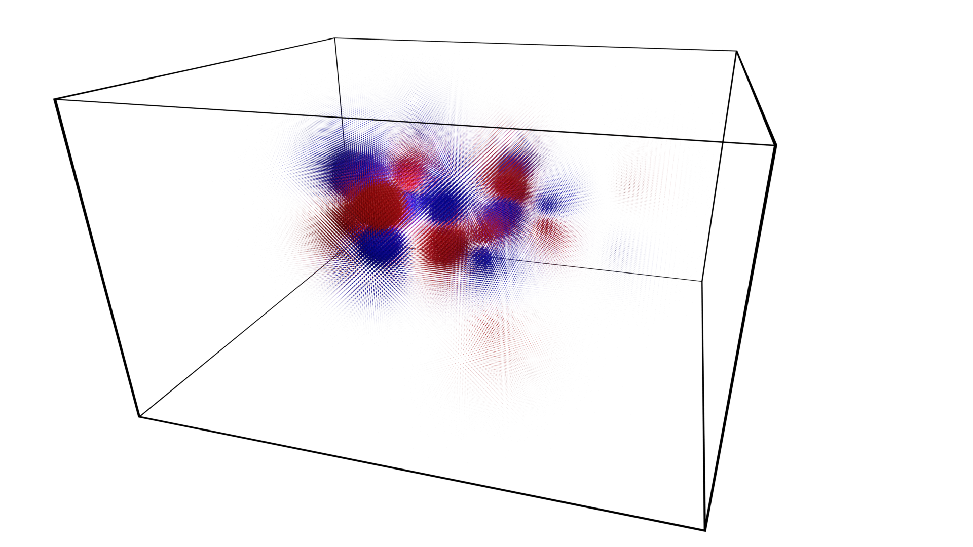
The package includes some example .cube data calculated for caffeine that has been rendered as a point cloud below.